Excel Sales Report (Part 3)-Pivot Tables

Now it’s time to create our reports using standard pivot tables. A pivot table creates calculations based on criteria and conditions. For the first report, I want to get Year Month sales.

To start, I click any cell in the flat table report and go to the Insert tab and select Pivot Table. Note -the shortcut Alt + N + V can also be used to insert a Pivot table.

Cell selected inside table indicated with bold green outline

Location of Insert tab and Pivot Table icon inside the ribbon

The following pop up screen appears after selecting Pivot Table

entire table is selected in preparation to create pivot table

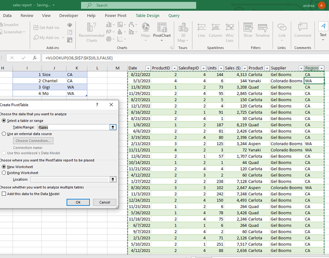
I selected Existing Worksheet and clicked in a cell on the new worksheet I created called Year Month Sales.

Destination information for pivot table

Empty pivot table

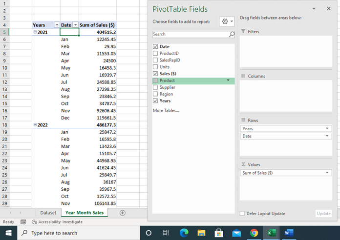
I dragged the field names into the criteria windows to create the pivot table report.

Pivot table before any formatting

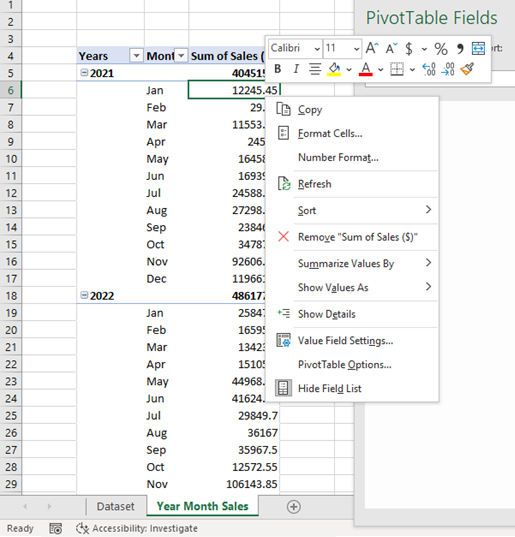
The date column is showing Sales on the daily basis, but I want to show Sales by Year and Month. Some versions separate the date automatically. My version does not, so I have to group. I right click on of the date cells in the pivot table and select grouping.

Selecting the grouping display for pivot table report

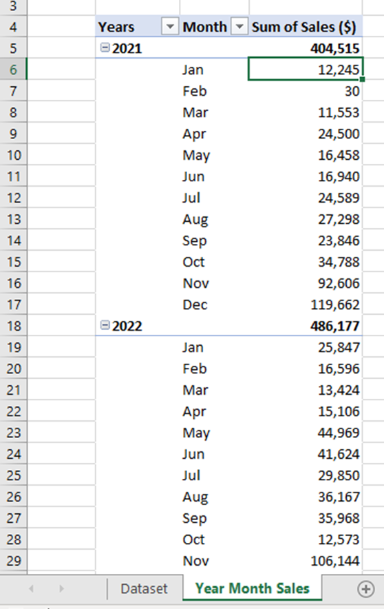
After selecting Years and Months, my pivot table updates to the correct break down for my report. Notice in the Rows that Years and Date are now populated.

Pivot table broken down into Year and Month

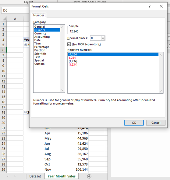
Because this is a standard pivot table vs a data model pivot table I have to manually format the numbers and change the date title.

Selecting Number Format

Formatting numbers

Numbers formatted and Date changed to Month

This completes the first pivot table report. Be sure to check out Part 1 and Part 2. And stay tuned for Part 4.